The simple linear model

In the previous chapter we started getting down to the nitty-gritty of the linear model that we've been discussing since way back in Chapter 2. We saw that if we wanted to look at the relationship between two variables we could use the model in equation (2.3):

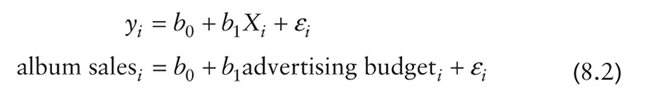
In this model, b is the correlation coefficient (more often denoted as r) and it is a standardized measure. However, we can also work with an unstandardized version of b, but in doing so we need to add something to the model:

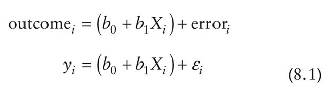
The important thing to note is that this equation keeps the fundamental idea that an outcome for a person can be predicted from a model (the stuff in brackets) and some error associated with that prediction (ε_i). We are still predicting an outcome variable (y_i) from a predictor variable (X_i) and a parameter, b₁, associated with the predictor variable that quantifies the relationship it has with the outcome variable. This model differs from that of a correlation only in that it uses an unstandardized measure of the relationship (b) and consequently we need to include a parameter that tells us the value of the outcome when the predictor is zero.¹ This parameter is b₀.

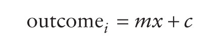
Focus on the model itself for a minute. Does it seem familiar? Let's imagine that instead of b₀ we use the letter c, and instead of b₁ we use the letter m. Let's also ignore the error term for the moment. We could predict our outcome as follows:

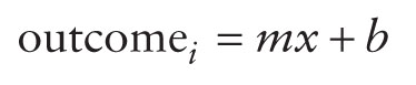
Or if you're American, Canadian or Australian let's use the letter b instead of c:

Perhaps you're French, Dutch or Brazilian, in which case let's use a instead of m:

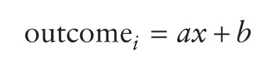
Do any of these look familiar to you? If not, there are two explanations: (1) you didn't pay enough attention at school, or (2) you're Latvian, Greek, Italian, Swedish, Romanian, Finnish or Russian - to avoid this section being even more tedious, I used only the three main international differences in the equation above. The different forms of the equation make an important point: the symbols or letters we use in an equation don't necessarily change it.² Whether we write mx + c or b₁X + b₀ doesn't really matter, what matters is what the symbols represent. So, what do the symbols represent?

Hopefully, some of you recognized this model as 'the equation of a straight line'. I have talked throughout this book about fitting 'linear models', and linear simply means 'straight line'. So, it should come as no surprise that the equation we use is the one that describes a straight line. Any straight line can be defined by two things: (1) the slope (or gradient) of the line (usually denoted by b₁); and (2) the point at which the line crosses the vertical axis of the graph (known as the intercept of the line, b₀). These parameters b₁ and b₀ are known as the regression coefficients and will crop up time and time again in this book, where you may see them referred to generally as b (without any subscript) or bn (meaning the b associated with variable n). A particular line (i.e., model) will have a specific intercept and gradient.

Figure 8.2 shows a set of lines that have the same intercept but different gradients. For these three models, b₀ will be the same in each but the values of b₁ will differ in each model.

Figure 8.2 also shows models that have the same gradients (b₁ is the same in each model) but different intercepts (the b₀ is different in each model). I've mentioned already that b₁ quantifies the relationship between the predictor variable and the outcome, and Figure 8.2 illustrates this point. In Chapter 6 we saw how relationships can be either positive or negative (and I don't mean whether or not you and your partner argue all the time). A model with a positive b₁ describes a positive relationship, whereas a line with a negative b₁ describes a negative relationship. Looking at Figure 8.2 (left), the red line describes a positive relationship whereas the green line describes a negative relationship. As such, we can use a linear model (i.e., a straight line) to summarize the relationship between two variables: the gradient (b₁) tells us what the model looks like (its shape) and the intercept (b₀) tells us where the model is (its location in geometric space).

This is all quite abstract, so let's look at an example. Imagine that I was interested in predicting physical and downloaded album sales (outcome) from the amount of money spent advertising that album (predictor). We could summarize this relationship using a linear model by replacing the names of our variables into equation (8.1):

Once we have estimated the values of the bs we would be able to make a prediction about album sales by replacing 'advertising' with a number representing how much we wanted to spend advertising an album. For example, imagine that b₀ turned out to be 50 and b₁ turned out to be 100. Our model would be:

Note that I have replaced the betas with their numeric values. Now, we can make a prediction. Imagine we wanted to spend £5 on advertising, we can replace the variable 'advertising budget' with this value and solve the equation to discover how many album sales we will get:

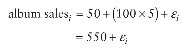
So, based on our model we can predict that if we spend £5 on advertising, we'll sell 550 albums. I've left the error term in there to remind you that this prediction will probably not be perfectly accurate. This value of 550 album sales is known as a predicted value.

---

¹ In case you're interested, by standardizing b, as we do when we compute a correlation coefficient, we're estimating b for standardized versions of the predictor and outcome variables (i.e., versions of these variables that have a mean of 0 and standard deviation of 1). In this situation b₀ drops out of the equation because it is the value of the outcome when the predictor is 0, and when the predictor and outcome are standardized then when the predictor is 0, the outcome (and hence b₀) will be 0 also.

² For example, you'll sometimes see equation (8.1) written as Y_i = (b₀ + b₁X_i) + e_i. The only difference is that this equation has bs in it instead of bs. Both versions are the same thing, they just use different letters to represent the coefficients.